🚀 Motivation
In our previous post, we explored how MATSim can simulate ride-hailing services using real-world data from Chicago’s TNP dataset. But ride-hailing is just one piece of the puzzle. What happens when we now transition the focus to ride-pooling, where multiple passengers share a vehicle?
Ride-pooling-based DRT systems bring a set of unique advantages that are often overlooked — especially in discussions around autonomous driving. While autonomy promises to revolutionize mobility, it’s equally important to rethink the operational models that go hand-in-hand with it. Choosing a service form that balances directness (as in taxis or private cars) with the ability to aggregate demand is key to building sustainable transport systems.
Traditional public transport excels in dense urban cores, where fixed routes and high frequencies make it efficient. However, in everyday life — especially for tangential trips in suburban areas or inter-village travel — conventional transit often falls short by design. It’s simply not optimized for these kinds of trips.
This article aims to serve as a starting point for anyone interested in simulating and evaluating ride-pooling systems in MATSim. At the same time, it’s a reminder of the transformative potential of ride-pooling: a mode that can dynamically adapt to demand, reduce fleet sizes, and bundle vehicle kilometers — all while offering a user experience that remains competitive with private car travel.
🧭 What is Ride-Pooling?
Ride-pooling refers to a mobility service where multiple passengers with similar routes share a single vehicle. Unlike traditional ride-hailing, which serves one passenger or group per trip, ride-pooling dynamically matches riders in real time to optimize vehicle occupancy and reduce redundant trips. Ride-pooling is often seen as a bridge between private ride-hailing and public transit — offering flexibility while improving efficiency. While ride-pooling promises significant benefits — such as reduced traffic, lower emissions, and better vehicle utilization — it also introduces new layers of complexity:
- How do we match passengers efficiently in real time?
- How much detour is acceptable before user satisfaction drops?
- How does pooling affect fleet size and total vehicle kilometers traveled (VKT)?
These questions are not just technical — they have direct implications for operational cost structures. For instance, pooling may reduce the number of trips but increase the duration and routing complexity of each ride. Conversely, ride-hailing may be simpler to operate but less efficient in terms of vehicle usage.
This post builds on the previous ride-hailing setup and demonstrates how a ride-pooling simulation can be implemented in MATSim. We provide example code, discuss key parameters, and share insights from a representative scenario in Chicago.
🧩 Setup: Defining a Ride-Pooling Service in MATSim
In our experience, the major core elements of a ride-pooling service definition are:
- The stop network (PuDo locations)
- The detour-determining constraints
- The rebalancing parametrization
- The vehicle and fleet size
🛠️ Generating Pick-Up and Drop-Off Locations
A critical component of comfortable ride-pooling simulations in MATSim is the creation of a pick-up and drop-off (PuDo) locations. The objective is to ensure that no passenger needs to walk farther than a configurable maximum distance to reach a stop. The following approach outlines how such a network is systematically generated.
The process begins by scanning all links in the MATSim network that support the "car" mode. For each eligible link, the generator calculates the number of stops required based on the link’s length and a configurable parameter called maxWalkDistance. These stops are then placed at evenly spaced intervals along the link geometry, using linear interpolation between the coordinates of the link’s nodes. This ensures that stop density reflects the physical layout of the road network and provides equidistant access for passengers.
To avoid redundant coverage, a spatial deduplication step is performed using a QuadTree data structure. All initially generated stops are inserted into the tree, and any new stop that falls within maxWalkDistance of an existing one is discarded. This guarantees spatial uniqueness while maintaining the goal of universal accessibility within walking distance.
Finally, the filtered set of stops is converted into TransitStopFacility objects, each retaining its associated link ID and coordinates. The resulting stop network is exported as a MATSim transit schedule and can be directly integrated into Demand Responsive Transport (DRT) simulations, enabling realistic modeling of ride-pooling systems.

📁 The code can be found and tested in the example repository . The result is a well-structured, spatially balanced stop network that builds the foundation of our ride-pooling analysis.
⚙️ Configuring Ride-Pooling Parameters
When setting up a ride-pooling service in MATSim, a wide range of parameters define how flexible, efficient, and user-friendly the system behaves. These parameters influence travel time, waiting time, and detour tolerance — all of which directly affect both passenger satisfaction and operational performance.
Since around 2017/18 and the first ride-pooling implementation by Joschka Bischoff et al., intensive development efforts — especially by contributors from MOIA, Volkswagen, and IRT SystemX — have led to a highly functional and robust DRT code base. The resulting implementation meets even the demanding requirements of industrial-scale applications, making MATSim one of the most versatile platforms for simulating demand-responsive transport systems.
While the following list of configuration options is far from exhaustive, it offers a first glimpse into the level of detail and realism with which DRT systems can be modeled in MATSim. From routing strategies and vehicle assignment logic to dynamic rebalancing and user-centric constraints — the simulation framework provides fine-grained control over nearly every aspect of ride-pooling operations.
MaxTravelTimeAlpha
This parameter defines how much longer a pooled ride may take compared to a direct trip. It acts as a multiplier on the shortest possible travel time. A higher value allows for more detour flexibility, enabling better pooling but potentially increasing passenger travel time.MaxTravelTimeBeta
This is an additive buffer that complements the alpha factor. It allows for a fixed amount of extra time on top of the proportional detour. Together, Alpha and Beta define the upper bound of acceptable travel time for pooled passengers.MaxWaitTime
This sets the maximum time a passenger is willing to wait for pickup after requesting a ride. It directly affects responsiveness and perceived service quality. Shorter wait times improve user experience but may reduce pooling efficiency.MaxAbsoluteDetour
This optional parameter defines a hard limit on the detour — either in time or distance — regardless of Alpha and Beta. It ensures that no passenger is excessively delayed due to pooling, acting as a safeguard for service reliability.
In this blogpost our team chose the following parameter combination to compare Ride Hailing and Ride Pooling
| Parameter | Ride Hailing | Ride Pooling |
|---|---|---|
| MaxTravelTimeAlpha | 1.0 | 1.5 |
| MaxTravelTimeBeta | 900 sec | 900 sec |
| MaxWaitTime | 900 sec | 900 sec |
| MaxAbsoluteDetour | - | 900 sec |
| OperationalScheme | door to door | stop based |
| PuDo Raster | - | 250 meters |
📊 Comparing Ride-Hailing and Ride-Pooling
🚗 Fleet Requirements
To assess the operational efficiency of ride-pooling, we conducted two MATSim simulations — one modeling a ride-hailing service and the other a ride-pooling service. Both scenarios were designed to serve exactly the same demand, as outlined in our previous post on DRT in Chicago.
In order to maintain a consistent service level, the target rejection rate was set to approximately 10% in both simulations. Fleet sizes were then calibrated accordingly to meet this benchmark.
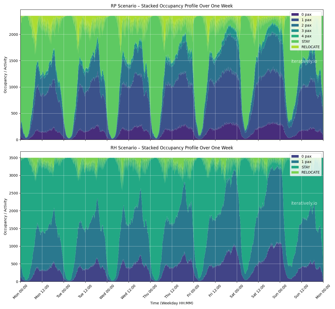
In the ride-hailing scenario, approximately 3500 vehicles were required to fulfill all requests. In contrast, the ride-pooling scenario achieved the same level of service with only 2350 vehicles. This represents a reduction of about 32.9% in fleet size, clearly demonstrating the potential of ride-pooling to improve vehicle utilization and reduce operational overhead.
The following figure illustrates the differences in fleet usage between the two scenarios:
⚠️ Note: In both simulations, each trip was modeled without additional passengers. Technically, MATSim supports multiple passengers per vehicle via DRT Companions, but due to the lack of concrete distribution data, our simulation assumed a consistent passenger-per-trip ratio across both systems.
📊 Mileage metrics
We focused on five core metrics that describe how the fleet moves through the network:
- Total Distance: Overall kilometers driven by the fleet.
- Empty Distance: Kilometers driven without passengers.
- Passenger Distance: Kilometers driven with passengers onboard.
- Empty Ratio: Share of empty distance relative to total distance.
- Average Driven Distance: Mean distance per vehicle.
These metrics were compared between RP and RH in the final iteration of the simulation.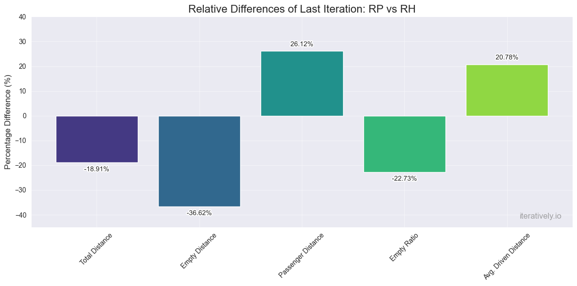
Ride Pooling demonstrates clear advantages over traditional Ride Hailing in terms of efficiency and vehicle utilization. The total distance driven by the RP fleet decreased by 18.91%, indicating that fewer kilometers were needed to serve demand—likely due to more optimized routing or a leaner fleet.
A particularly striking improvement is the 36.62% reduction in empty distance, showing that Ride Pooling significantly minimizes deadheading. This means vehicles spend much less time driving without passengers, which translates to lower operational costs and reduced traffic impact. This aspect is especially relevant for automated mobility services, where—unlike in gig-based models like Uber—the operator of the vehicle directly bears the cost of empty trips. In human-driven ride hailing, deadheading is often absorbed by the driver as part of their flexible work model. However, in autonomous fleets, every kilometer driven without a passenger becomes a direct financial burden for the operating company.
This shift in cost responsibility could become a strategic incentive for mobility providers to transition toward pooling-based services. Especially in markets like the United States, where ride hailing is deeply embedded in urban mobility, operators may increasingly seek to encourage pooled rides—potentially through more attractive pricing models—to reduce inefficiencies and improve fleet economics.
At the same time, RP vehicles covered 26.12% more kilometers with passengers onboard, suggesting either higher demand or better service coverage. The empty ratio also dropped by 22.73%, confirming that a larger share of vehicle movement is now productive, with passengers on board.
However, this efficiency comes with a trade-off: the average distance driven per vehicle increased by 20.78%. Each vehicle now travels significantly more kilometers per day, which could imply longer shifts, larger service areas, or fewer vehicle rotations—factors that may affect maintenance cycles, energy consumption, and operational planning, especially in autonomous or electric fleets.
🧠 Strategic Implications for Operators
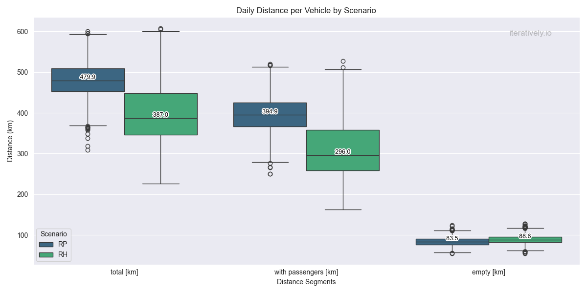
Based on the previously calculated daily mileage—480 km for Ride Pooling (RP) and 380 km for Ride Hailing (RH)—the following first rough strategic assessments can be made regarding fleet planning and cost structures for mobility operators.
While RP vehicles reach their planned lifetime of 300,000 km roughly 164 days sooner due to higher daily usage, this is offset by the fact that RP systems require approximately 30% fewer vehicles to serve the same demand. This fundamental difference leads to several important strategic implications:
- Lower initial investment: The reduced fleet size in RP systems results in significantly lower upfront capital expenditures.
- Better utilization: RP vehicles spend considerably less time driving without passengers (−36.62% empty distance), which improves operational efficiency and reduces costs.
- Reduced traffic impact: More passenger kilometers are delivered with fewer vehicles on the road, contributing to less congestion and lower emissions.
- Strategic fit for automation: In autonomous fleets, deadheading becomes a direct cost to the operator—not the driver. RP’s ability to minimize empty trips is therefore economically critical.
- Optimized replacement cycles: Although RP vehicles wear out faster due to higher daily mileage, the smaller fleet size leads to lower annual replacement costs compared to RH.
🙋♂️ User Perspective
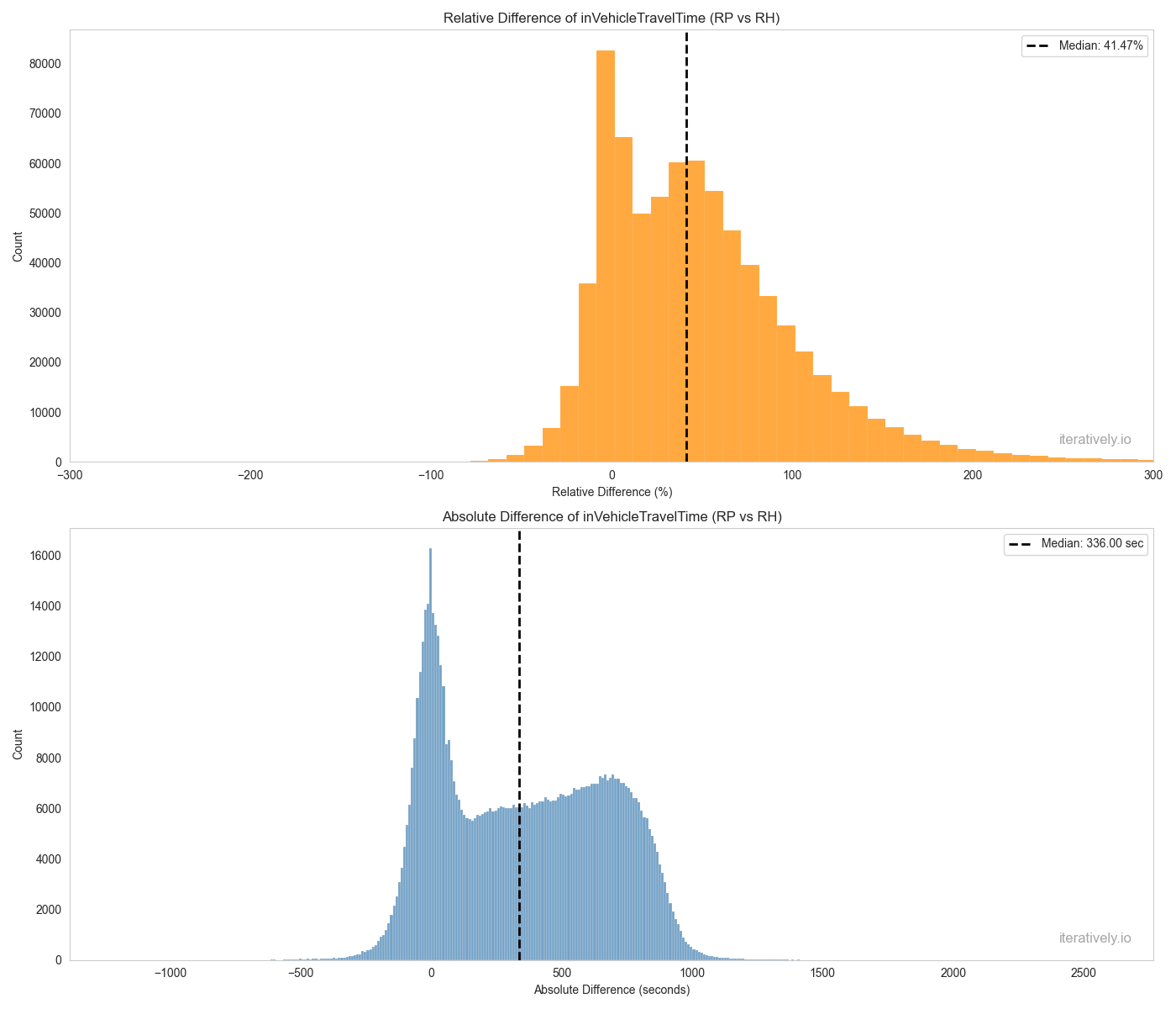
Building on the operator-focused analysis, we now transition to the user perspective, which is equally crucial when evaluating the viability of Ride Pooling (RP) systems. The simulation results reveal that passengers in RP spend, on average, 336 seconds (about 5.6 minutes) longer in the vehicle compared to traditional Ride Hailing (RH). In relative terms, this corresponds to a 41.47% increase in travel time.
This extended in-vehicle time is a natural consequence of pooling, where multiple passengers with similar destinations are grouped into shared trips. While this may seem like a drawback at first glance, it opens up several user-centric advantages. The most obvious is lower cost per ride, as the operational expenses are distributed across more passengers. Additionally, pooling enables higher service availability, particularly during off-peak hours or in areas with lower demand density. It can also lead to shorter wait times, since the fleet is utilized more efficiently and vehicles are more likely to be nearby.
Despite the longer travel times, many users may find RP to be a compelling alternative—especially if the service is priced attractively and offers a reliable, comfortable experience. This highlights a key insight: user acceptance is critical. If passengers are willing to trade a few extra minutes for better prices and broader coverage, pooling can become a cornerstone of future urban mobility.
Operators can actively support this shift by ensuring transparent communication about expected travel times, offering competitive pricing models, and investing in vehicle comfort and routing reliability. These elements help build trust and make the service more appealing, even if the journey takes slightly longer.
Ultimately, this perspective reinforces the strategic value of agent-based mobility simulation with MATSim. It allows operators not only to optimize fleet operations and cost structures but also to evaluate and anticipate user experience—an essential factor in the success of any mobility service. By simulating real-world behavior and system dynamics, MATSim empowers decision-makers to balance efficiency, cost, and satisfaction in a data-driven way—before a single vehicle hits the road.
Author: Steffen Axer